Graphical abstract
Abstract
Electrification has allured policy makers as the “most” compelling solution to reduce GHG emissions. Almost all of the government actions envision this trend. Indeed, the global energy system is facing a massive electrification of energy end-uses that associated with a deep decarbonisation of the power sector, has been identified as a key strategy to accelerate the transition to low-carbon energy systems. However, there remains a lack of comprehensive analysis of the key enablers to trigger such a change. In this paper, we explore how the electrification rate will affect the emissions trends by 2050 and how it will impact the overall efficiency of the system. Our results show the potential of electrification opportunities and main drivers for transport, buildings and industry. While this trend clearly improves the way we use final energy - energy efficiency in final use, for most of the scenarios studied, higher electrification rates also make growth the conversion losses between final over primary energy transformation, reducing the overall efficiency of the system. A balance between these two trends much be carefully examined, in order to determinate how the electrification share in final energy used impacts on the total energy system efficiency.
Main
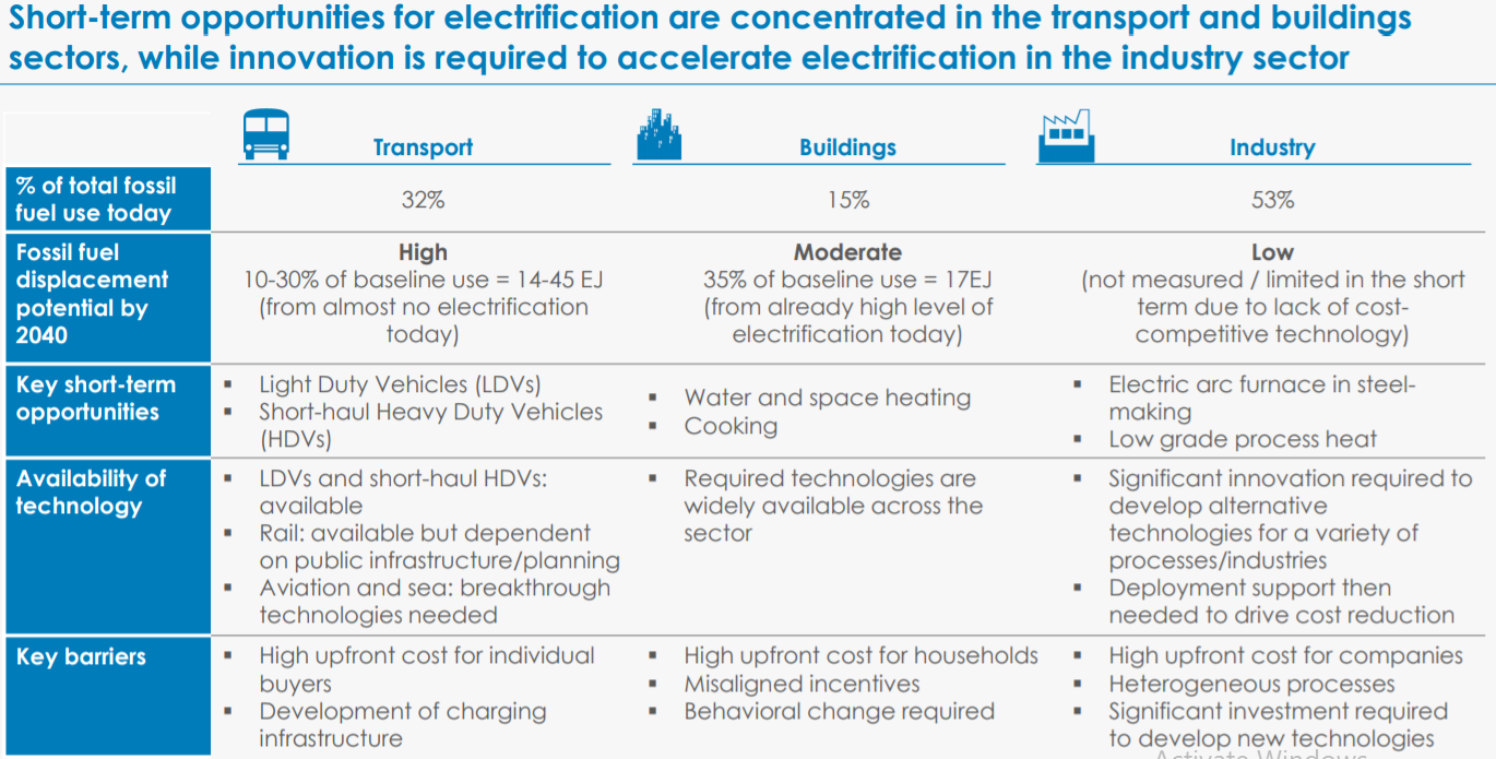
Decarbonization of power combined with electrification is identified as a major transition strategy towards low-carbon energy systems . Extended electrification of end-uses is therefore expected to play an important role in substituting fossil fuels and reducing CO2 emissions . This idea has allured policy makers as one of the most compelling for GHG mitigation. Many studies assess electrification potentials at the sectoral level . Most of them agree that transport is the end-use sector with the highest potential, followed by buildings; on the other hand, industry seems more difficult to electrify. Fewer studies evaluate electrification prospects across all end-uses , and even fewer at the global level. Scarce evidence indicates potential savings of CO2 emissions of up to 2-4 GtCOCO2 in the next 20-30 years.
One key question remains related to the driving forces of such a transition process. From a historical perspective, factors such as end-use services and energy prices, consumers acceptance factors or industrial dynamics play an important role to trigger and sustain transition processes . On the other hand, adequate policy interventions might not be produced unless thought in conjunction with consumers’ behaviours. Such considerations call for a deeper analysis of the driving forces behind energy systems’ electrification, accounting for such effects, but also exploring the consequences of electrification on the energy landscape. Indeed, systems effects of electrification may extend beyond GHG emissions mitigation, especially when looking at the system from a holistic efficiency perspective.
"Such considerations call for a deeper analysis of the driving forces behind energy systems’ electrification"
The present study is an attempt to address at the global level the triple objective of identifying (i) the potential for electrification (ii) the main drivers for unlocking electrification potential at the global and sectoral levels and (iii) some system-wide consequences of advanced electrification. Our results indicate that depending on the prevailing economic and behavioural conditions, electricity consumption could represent between 3.5 and 5 Gtoe/yr in 2050, which corresponds to 30 to 50% of total end-uses. Climate policies and non-economic factors will play a crucial role to electrify end-uses, before energy prices and technologies costs. We confirm that transport, before buildings and industry, has a crucial role to play among all end-uses to foster the use of electricity. However, its potential might be difficult to fully exploit, because it evenly depends on a variety of factors. Therefore, adequate policy frameworks should address multiple dimensions at once. Finally, we highlight a potential trade-off in terms of efficiency, since electrification displaces direct uses of fossil fuels in favour of a secondary energy vector. We suggest that this loss of upstream energy efficiency might be compensated by important end-use efficiency gains in the main consuming sectors.
Scenarios
We identified five groups of drivers potentially affecting the level of electrification of the energy system: climate policy, energy prices, energy supply technologies costs, end-uses technologies costs, and non-economic drivers. Each group contains one or several parameters; for each of them, we defined a “low electrification” (not in favour of electrification) and a “high electrification” (in favour of electrification) value – based to the extent possible on existing literature.
We designed a coherent set of 32 scenarios with the POLES-JRC model , a long-term, partial equilibrium model of the global energy system, covering the whole energy lifecycle from resources extraction to energy end-uses. These scenarios take the form of a binary tree, meaning that all “low electrification” and “high electrification” parameters values were run for the five assumptions groups:
- Climate policy includes a set of instruments aiming at driving the energy system along a 2C-compatible GHG emissions pathway. Carbon pricing is the main tool used for this purpose, along with energy taxes or incentives for energy efficiency.
- Primary energy prices on the primary supply side, different fossil fuel prices affect (on top of climate policies, especially carbon values) upwards or downwards the competitiveness of low-carbon energy sources and technologies, including those being used for power generation. The competitiveness of electricity as a final energy carrier crucially depends on the relative evolution of the price of fossil fuels specialised on power generation (e.g. coal) with respect to those with higher use as final energy carrier. Similarly, at end-use level, where electricity competes with natural gas and oil products in transport (in road mode in particular), residential and services (for cooking, space and water heating) and industry (process heat). Moreover, biomass prices are also likely to affect electricity uses, since they also compete with electricity for final demand. Sensitivity analyses on extraction costs will include changing oil, gas and biomass prices, all together, upwards (making electricity more competitive) or downwards (making electricity less competitive).
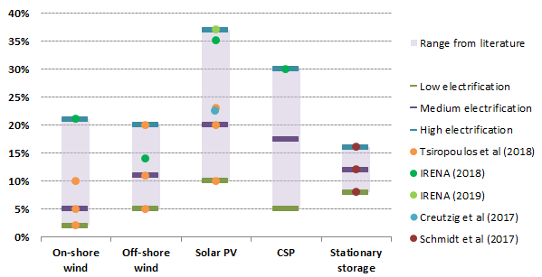
- Costs of electricity supply technologies unlike well-established fossil-fuel technologies, the future costs of low-carbon power generation options are subject to wide uncertainties. However, these assumptions play a key role in the assessment of the competitiveness of these technologies; this is especially true for investment costs, since these technologies have low variable costs. Recent literature reviews (see e.g. (Tsiropoulos, Tarvydas, & Zucker, 2018)) show, across different studies, a globally decreasing trend, especially for wind and solar technologies. Nevertheless, actual investment costs assumptions vary widely depending on the study. In turn, those costs will affect the average electricity prices, and in the end the competitiveness of electric end-use technologies. The POLES-JRC model uses a one-factor learning model to project future investment costs based on endogenously calculated cumulated installed capacities. Ranges for learning rates are taken from literature studies, assuming higher learning rates (i.e., rapidly falling investment costs) in the high electrification scenario.
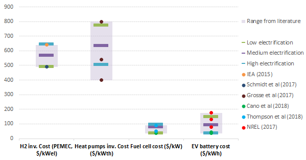
- Costs of electric end-use technologies Energy prices will affect the running costs of energy equipment; and relatively cheaper carbon-free electricity is crucial to deliver a higher electrification shares, but not the only one. A key driver to unlock the potential of electricity in end-uses is lies on electric end-use costs and their relative competitiveness with non-electric ones. Assumptions were made on the costs of heat pumps, batteries for electric vehicles and hydrogen fuel cells, which are uncertain and may deeply affect consumers' choices. In an energy system becoming more efficient, the cost structure of energy expenditures is likely to give more weight to fixed costs as opposed to variable costs (European Commission, 2018). Moreover, some electricity technologies have an important potential in terms of efficiency compared to conventional ones (e.g. heat pumps, electric vehicles). This sensitivity analyses section shall provide some conclusions on the underlying cost/efficiency trade-off.
- Technology adoption dynamics and other non-economic drivers. This fourth group of parameters includes important consumer behaviour parameters, as well as some institutional ones. Beyond economic indicators, many drivers may affect economic agents' decisions to use electricity, but are essentially not covered by the economic mechanisms endogenously described in POLES-JRC. This applies to some political choices (promoting some industrial pathways, regulating operations in energy production/generation/distribution, investment in electric vehicles recharging infrastructure, etc.), to consumer adoption dynamics (evolving preferences related to advertisement, exposure levels, etc., (Sterman, 2000), (Struben & Sterman, 2008), and finally also to other behaviour-related elements (such as the propensity to adopt new information technologies and respond to economic signals to manage electric load, etc…).
"We vary technological, behavioural, economical and policy assumptions to produce a comprehensive set of scenarios"
For example, testing all scenarios combinations between no carbon and 2°C compatible carbon policy one the one side, and low or high energy prices on the other side, would bring 4 scenarios. With 5 groups of assumptions, we end up running $2^{5}=32$ scenarios, up to 2050.

Figure. Scenarios design.
We end up with 2 extremes scenarios, one “Low Electrification” or “No effects”, for which all parameters of each group take a value preventing electrification, and a “High Electrification” or “All effects”, for which all parameters of each group take a value in favour of electrification.
"We use a well-established cooperative game-theoretic concept, the Shapley Value, to distribute the impact of assumptions on model outcomes"
This experiment is designed as a structured scenario tree, so that $N$ scenario groups are tested according to binary choices (No/Yes, Low/High etc...), which we encode as $\{0,1\}^{N}$, for the sake of brevity. It is relevant to examine the contribution of each scenario group to the change of a given model outcome. For example, how much does each policy affect the overall electrification of the energy system? Intuitively, it seems that it should involve the comparison between the scenarios $\{0\}^{N}$ and $\{1\}^{N}$. The underlying problem consists in being able to identify -- given that policy overlaps (synergies but also antagonistic effects) exist -- those policies that are potentially more effective with respect to the chosen metrics. Since the corresponding effects are likely to be nonlinear\footnote{And nonconvex, hence monotonicity in the effects is not guaranteed.}, there is no obvious, unique way to perform such an allocation. Besides, it is very likely that the effect of a given assumption along the tree may be different depending on the values taken on the other branches. Therefore, a meaningful allocation procedure should involve not only the extreme combinations to be compared ($\{0\}^{N}$ and $\{1\}^{N}$), but all their intermediates in the set $S=\{00...0,...,11...1\}$, whose cardinality is $|S|=2^{N}$.
To distribute the effects of any assumptions group on any output variable or indicator, using a well-established cooperative game-theoretic concept, the Shapley Value. Indeed, the binary scenarios tree defined here is equivalent to a n-person cooperative, transferable utility game -- where scenario groups are the players, and the value function is the model output. Calculating all groups combinations allows to determine the incremental value of all groups, in all sequences ; the Shapley value consists in averaging the incremental value of each group over all possible permutations to obtain the complete coalition. The general formulation of the Shapley value for an N-players game is \begin{equation} \varphi_{i}(v) = \sum_{S\subseteq N}\frac{(|N|-|S|)!(|S|-1)!}{|N|!}(v(S)-v(S\diagdown\{i\})) \end{equation} where
- $\varphi_{i}(v)$ is the Shapley Value of group $i$ for the value function $v$;
- $S$ is a subset of groups.
Global electrification trends and their drivers, and related emissions
First, consider global end-use electrification trends at the world level by 2050. Electrification is measured using different metrics, (i) the absolute total final electricity demand and (ii) the share of electricity consumption over total final energy demand. The purpose of using these two different metrics is to investigate the interplay between total energy demand and electrification, in the sense that an increased market share of electricity in final uses does not necessarily imply a higher electricity consumption, because of other measures which could affect global consumption patterns, especially energy efficiency.
Figure. (a1) World total final electricity consumption in Gtoe/yr between 1990 and 2050, all scenarios range (grey shaded), median (black), no effects (purple), all effects (green), and IAMC1.5C scenarios 95% confidence interval range (orange). (a2) Shapley decomposition of total final electricity consumption (from no effects scenario to all effects scenario). (b1) World share of electricity in total final energy consumption between 1990 and 2050, all scenarios range (grey shaded), median (black), no effects (purple), all effects (green), and IAMC1.5C scenarios 95% confidence interval range (orange). (b2) Shapley decomposition of share of electricity in total final energy consumption (from no effects scenario to all effects scenario). (c) World total final energy consumption (Gtoe) in 2050 (x-axis) vs world share of electricity in total final energy consumption (%) in 2050 (y-axis); colors are scaled to the world total final electricity consumption (Gtoe) in 2050, all scenarios.
Figure shows the results for the two metrics, at the world level, along with a comparison with existing literature and their Shapley value decomposition. We find (panel a1) a total final electricity consumption ranging from 3.6 to 5.2 Gtoe/yr in 2050, compared to 1.7 Gtoe in 2015, and less than 1 in 1990. This falls within the range of the IAMC 1.5 Scenario Explorer dataset, although covering less than half of the range. In terms of growth rates, we generallyobtain (except for a handful of scenarios), lower values for the projection period (2015-2050; median at 2.71%/yr, 75th percentile at 2.92%/yr, maximum at 3.20%/yr) than for history (1990-2015; 2.95%/yr): the pace of growth of electricity consumption can be expected to be lowering. This suggests that although policies, behavioural and technological changes are to be applied, a large proportion of the electrification has been done in the past (consistent with Mai et al (2018), see Morton (2002), Fouquet (2016), Tsao et al (2018)). The No effects and All effects scenarios are not the lowest and highest trajectories, but are intermediate scenarios, indicating that assumptions groups play either a positive or a negative role in the total electricity consumption (panel a2). Indeed, climate policies affect electricity consumption negatively; they are responsible for about -0.5Gtoe/yr in 2050. The underlying mechanism relies on the energy and non-energy efficiency measures triggered by climate policies. Carbon pricing implies a stabilization of even a drop in the total final energy consumption, therefore pushing electricity consumption down. On the other hand, non energy factors, demand and supply technologies costs contribute to increasing electricity consumption, as much as 0.6, 0.5 and 0.1 Gtoe/yr respectively. Such drivers have a smaller perimeter than climate policies; they target electric technologies and consumption directly. Finally, primary energy prices have a minor negative impact on electricity consumption, channeled through their positive impact on non-free fuel based electricity production costs.
In terms of market share, our results indicate that electricity could cover between 31 and as high as 51% of the final energy needs in 2050 (panel b1); the median scenario reaches 40% of electricity in final uses in 2050. This is again consistent with the current body of literature. In addition, using the market share as an electrification metric, the No effects and All effects scenarios indeed correspond to the low and high electrification pathways. In this case, all of the scenarios assumptions groups positively contribute to an increase in electrification (panel b2), with a prominent role of climate policies (+8.4%), before non-energy drivers (+6.3%), end-use technologies costs (+2.5%), primary energy prices (+2.1%) and energy supply technologies costs (+0.7%)."Electrification does not necessarily imply an increase in electricity consumption."
The comparison of the two metrics reveals an interesting pattern for understanding future electrification dynamics. Consistently with other research (Sugiyama, 2012), we conclude that an increase of the electricity market share does not necessarily imply an increase of electricity consumption. Indeed, the market share of electricity can increase although the absolute consumption goes down, as long as the consumption of other fuels is more impacted. This mechanism is highlighted in panel c. High electrification shares are obtained for low total final energy consumptions, but higher electricity consumptions can be obtained for intermediate electrification shares and higher total energy demands. The fundamental driving force of this ambiguity is the climate policy, followed by energy prices. Both drivers are allocated a negative impact on electricity consumption, but a positive one on market shares. This means that such drivers, which are characterized by a wider base than electricity-targeted components, affect direct fuel uses more than electricity.
An interesting question to tackle relates to the consequences of electrification in terms of CO2 emissions. The current status of research points towards a clear correlation between electrification and CO2 emissions, which we aim at investigating now (Figure).
Figure. (a) World total energy-related CO2 emissions in GtCO2/yr between 1990 and 2050, all scenarios range (red shaded, without climate policy; blue shaded, with climate policy), no effects (purple), all effects (green). (b1) World total energy-related CO2 emissions by sector in 2018. (b2) World total energy-related CO2 emissions by sector in 2050, no effects scenario. (b3) World total energy-related CO2 emissions by sector in 2050, all effects scenario. (c) Contributions to world total energy-related CO2 emissions in 2050.(d) World share of electricity in total final energy consumption (%) in 2050 (x-axis), vs world total energy-related CO2 emissions in 2050 (y-axis); colors are scaled to the world total final electricity consumption (Gtoe) in 2050, all scenarios.
In 2018, the total energy-related CO2 amounted to 33.5 Gt (panel a), out of which more than one third due to power generation, 22% to transport, 19% to industry and 10% to both residential and services buildings (panel b1). The evolution of emissions over time splits into two groups, without and with climate policy. Within these groups, the No effects and All effects scenarios reach 47 and 9GtCO2, respectively. The obvious, expected role of climate policies in mitigating emissions is as high as -34GtCO2 (panel c). Other factors contribute to second-order, deeper cuts: energy supply technonologies costs provide, compared to this amount, a small contribution of -3GtCO2, and non-energy drivers contribute to less than 1GtCO2. Therefore, the spread of emissions within each climate policy group is reduced; however, there is more room for other effects to achieve deeper cuts without climate policy, to save up to 8 GtCO2 in 2050 (against 3.5 with climate policy). Another importan feature relates to the distribution of emissions across sectors; reducing emissions come along with a strong decarbonization of the power sector under climate policies, from more than one third (largest emitter) to less than 20% of total energy-related emissions in the All effects scenario (panel b3). Conversely, in the No effects scenario, both emissions and the share of power generation in emissions increase.
We then try to corroborate existing results from the literature and link electrification, expressed as the share of electricity in total final energy consumption, with CO2 emissions, as shown in panel d. If we summarize each of the two scenarios groups with and without climate policy, using e.g. the median, we observe a simple negative link between emissions and electrification. This simple correlation is consistent with other studies, but says little about the actual causal
relationships between these system-wide variables. Our experimental results do reveal more complex patterns. The ensemble of scenarios produced in this study can be split into three groups. Low electrification levels (31-36% in 2050) are associated with high emissions and average electricity consumptions (4.2-4.6 Gtoe in 2050). Scenarios with intermediate electrification levels (38-44% in 2050) correspond to either high emissions and electricity consumptions, or low emissions and electricity consumptions. Finally, high electrification is only associated to low emissions, and electricity consumptions ranging between 4.4 and 4.8 Gtoe in 2050. These results highlight some of the many possibilities to achieve similar emissions mitigation objectives. Once controlling for the effect of the climate policy, we hardly find a correlation between electrification and emissions; we observe that several sets of scenarios provide similar emissions but very different levels of electrification. This suggests an important observation with respect to the system's behaviour, namely that rather than electrification causing emissions reductions, both factors are cofounded by other drivers, such as climate policies or technologies. To confirm this result, we performed a simple causal inference test between electrification and emissions, and found no statistical evidence of a direct causal link. Only in the case of no climate policy and low energy supply technologies costs, do we find that increasing electrification from 31 to 43% saves about 2.5GtCO2, a result again consistent with other studies (Copenhagen economics, 2017)."Electrification and CO2 emissions mitigation are partly cofounded by climate policies"
Electrification throught the system efficiency lens
The effect of electrification and its drivers on the macro-behaviour of the energy system can be analysed using a simple Kaya decomposition of the total final energy consumption, as the product of population, GDP per capita, primary energy intensity of the economy and overall final to primary system efficiency, $TFEC_{t}=POP_{t}\frac{GDP_{t}}{POP_{t}}\frac{TPES_{t}}{GDP_{t}}\frac{TFEC_{t}}{TPES_{t}}$, or $TFEC_{t}=POP_{t}GDPP_{t}PEI_{t}\epsilon_{t}$. This decomposition highlights the role of primary energy intensity and overall syste efficiency in the evolution of final energy consumption.
Figure. (a1) World primary energy intensity (ktoe/MUSD) between 1990 and 2050, all scenarios range (grey shaded), median (black), no effects (purple), all effects (green). (a2) Shapley decomposition of world primary energy intensity (from no effects scenario to all effects scenario). (b1) World final over primary energy efficiency between 1990 and 2050, all scenarios range (grey shaded), median (black), no effects (purple), all effects (green). (b2) Shapley decomposition of final over primary energy efficiency (from no effects scenario to all effects scenario).
Comments to be written.
A synthetic theory of efficiencies
The ambiguous behaviour of global system efficiency can be explored further, using an analytical approach. It can be expressed as \begin{equation} \eta_{O}=\eta_{E}\sigma_{E}^{P}+\eta_{NE}(1-\sigma_{E}^{P}), \end{equation} where $\eta_{O}$, $\eta_{E}$ and $\eta_{NE}$ are the overall, electric and non-electric system efficiencies, respectively; $\sigma_{E}^{P}$ is the share of primary electricity devoted to power generation. All variables are time-dependent, and the time subscripts are omitted for simplicity. This equation can be further decomposed as follows: \begin{equation} \eta_{O}=[\eta_{RE}\sigma_{RE}^{P}+\eta_{NRE}(1-\sigma_{RE}^{P})]\sigma_{E}^{P}+[\eta_{S}\sigma_{S}^{P}+\eta_{NS}(1-\sigma_{S}^{P})](1-\sigma_{E}^{P}), \end{equation} where $\eta_{RE}$, $\eta_{NRE}$, $\eta_{S}$ and $\eta_{NS}$ represent, respectively, the renewable electrical, non renewable electrical, synfuels qnd non-synfuels efficiencies; $\sigma_{RE}^{P}$ and $\sigma_{S}^{P}$ are the shares of primary inputs devoted to renewable power generation and synfuels production.
To explore the dynamics of change, we compute the time derivative for the overall efficiency: \begin{equation} \dot{\eta}_{O}=\underbrace{(\eta_{E}-\eta_{NE})\dot{\sigma}_{E}^{P}+(\eta_{RE}-\eta_{NRE})\sigma_{E}^{P}\dot{\sigma}_{RE}^{P}+(\eta_{S}-\eta_{NS})(1-\sigma_{E}^{P})\dot{\sigma}_{S}^{P}}_{\text{Effect of market dynamics at constant technological structure}} + \underbrace{[\dot{\eta}_{RE}\sigma_{RE}^{P}+\dot{\eta}_{NRE}(1-\sigma_{RE}^{P})]\sigma_{E}^{P}+[\dot{\eta}_{S}\sigma_{S}^{P}+\dot{\eta}_{NS}(1-\sigma_{S}^{P})](1-\sigma_{E}^{P})}_{\text{Effect of technological change at constant market structure}} \end{equation}
Figure. (a) Electrical (bottom) and non electrical primary-to-final conversion efficiencies between 1990 and 2050, all scenarios range (grey shaded), median (black), no effects (purple), all effects (green). (b) Synthetic fuels (synthetic liquids, synthetic gas, biofuels, hydrogen) production (x-axis, Gtoe) vs nonelectrical conversion efficiency (y-axis, %); colors represent climate policies or specific scenarios. (c) Efficiency pathways for a subset of scenarios by 2050: non electrical conversion efficiency (x-axis, %), electrical conversion efficiency (y-axis, %), share of primary input to power generation in total primary energy supply (size, %) and final electricity consumption (color, Gtoe).
Comments to be written.
Discussion
Annex - Methodology
The JRC-POLES model -- this is to be rewritten, because not straight to the point
For a fuller description of the model, see (Després, Keramidas, Schmitz, Kitous, & Schade, 2018).
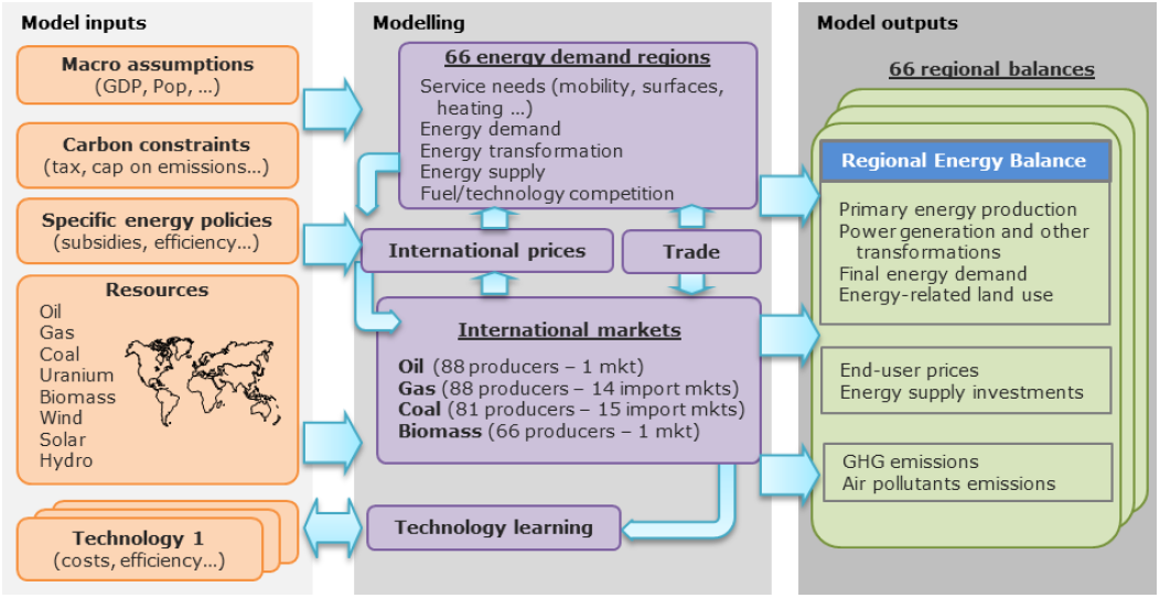
POLES-JRC is a world energy-economy partial equilibrium simulation model of the energy sector, with complete modelling from upstream production through to final user demand. It follows a year-by-year recursive modelling, with endogenous international energy prices and lagged adjustments of supply and demand by world region, which allows for describing full development pathways to 2050 (see general scheme in Figure 72).
The model provides full energy and emission balances for 66 countries or regions worldwide (including detailed OECD and G20 countries), 14 fuel supply branches and 15 final demand sectors. This exercise used the POLES-JRC 2019 version. Differences with other exercises done with the POLES-JRC model by EC JRC, or with exercises by other entities using the POLES model, can come from different model version, historical data sets, parameterisation, and/or policies considered.
Final demand
The final demand evolves with activity drivers, energy prices and technological progress. The following sectors are represented:
- industry: chemistry (energy uses and non-energy uses are differentiated), non-metallic minerals, steel, other industry;
- buildings: residential, services (detailed per end-uses: space heating, space cooling, water heating, cooking, lighting, appliances);
- transport (goods and passengers are differentiated): road (motorcycles, cars, light and heavy trucks; different engine types are considered), rail, inland water, international maritime, air (domestic and international);
- agriculture.
Power system
The power system describes the capacity planning of new plants and the operation of existing plants. The electricity demand curve is built from the sectoral distribution. 134 The load, wind supply and solar supply are clustered into a number of representative days. The planning considers the existing structure of the power mix (vintage per technology type), the expected evolution of the load demand, the production cost of new technologies and the resource potential for renewables. The operation matches electricity demand considering the installed capacities, the variable production costs per technology type, the resource availability for renewables and the contribution of flexible means (stationary storage, vehicle-to-grid, demand-side management). Electricity price by sector depend on the evolution of the power mix, of the load curve and of the energy taxes. Other transformation The model also describes other energy transformations sectors: liquid biofuels, coal-to-liquids, gas-to-liquids, hydrogen, centralised heat production.
Oil supply
Oil discoveries, reserves and production are simulated for producing countries and different resource types. Investments in new capacities are influenced by production costs, which include direct energy inputs in the production process. The international oil price depends on the evolution of the oil stocks in the short term, and on the marginal production cost and ratio of the Reserves by Production (R/P) ratio in the longer run.
Gas supply
Gas discoveries, reserves and production are simulated for individual producers and different resource types. Investments in new capacities are influenced by production costs, which include direct energy inputs in the production process. They supply regional markets through inland pipeline, offshore pipelines or LNG. The gas prices depend on the transport cost, the regional R/P ratio, the evolution of oil price and the development of LNG (integration of the different regional markets).
Coal supply
Coal production is simulated for individual producers. Production cost is influenced by short-term utilisation of existing capacities and a longer-term evolution for the development of new resources. They supply regional markets through inland transport (rail) or by maritime freight. Coal delivery price for each route depends on the production cost and the transport cost.
Biomass supply
The model differentiates various types of primary biomass: energy crops, short rotation crop (lignocellulosic) and wood (lignocellulosic). They are described through a potential and a production cost curve – information on lignocellulosic biomass (short rotation coppices, wood) is derived from look-up tables provided by the specialist model GLOBIOM-G4M (Global Biosphere Management Model). Biomass can be traded, either in solid form or as liquid biofuel.
Wind, solar and other renewables
They are associated with potentials and supply curves per country. GHG emissions CO2 emissions from fossil fuel combustion are derived directly from the projected energy balance. Other GHGs from energy and industry are simulated using activity drivers identified in the model (e.g. sectoral value added, mobility per type of vehicles, fuel production, fuel consumption) and abatement cost curves. GHG from agriculture and LULUCF are derived from GLOBIOM-G4M lookup tables.
Countries and regions
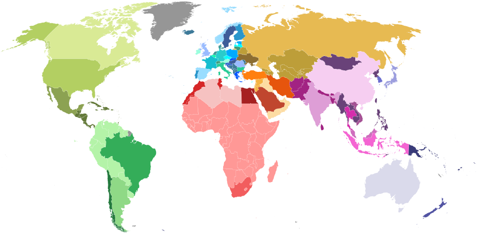
The model decomposes the world energy system into 66 regional entities: 54 individual countries and 12 residual regions (Figure 73, Table 14, Table 15), to which international bunkers (air and maritime) are added. 135
Understanding sensitivities with Shapley values
Some "well-defined" computational experiments are suitable for the use of specific ex-post methods to analyze the impact of the different scenarios dimensions on model outcomes.
Assume the experiment is designed as a structured scenario tree, so that $N$ scenario components are varied according to binary choices (No/Yes, Low/High etc...), which we encode as $\{0,1\}^{N}$, for the sake of brevity. Such dimensions can be "low or high oil price", "no subsidy or subsidy to electric vehicle".\
It is relevant to examine the contribution of each scenario branch to the change of a given model outcome. For example, how much does each policy affect the share of electric vehicles in the regional fleets? Intuitively, it seems that it should involve the comparison between the scenarios $\{0\}^{N}$ and $\{1\}^{N}$. The underlying policy problem consists in being able to identify -- given that policy overlaps (synergies but also balancing effects) exist -- those policies that are potentially more effective with respect to the chosen metrics. Since the corresponding effects are likely to be nonlinear\footnote{And nonconvex, hence monotonicity in the effects is not guaranteed.}, there is no obvious, unique way to perform such an allocation. Besides, it is very likely that the effect of a given assumption along the tree may be different depending on the values taken on the other branches. Therefore, a meaningful allocation procedure should involve not only the extreme combinations to be compared ($\{0\}^{N}$ and $\{1\}^{N}$), but all their intermediates in the set $S=\{00...0,...,11...1\}$, whose cardinality is $|S|=2^{N}$.
This problem is actually very frequent in economics; it occurs whenever an organisation -– a group of economic agents –- is willing to share some common costs or benefits across its entities or members. Those arise when infrastructures or services have to be commonly built and/or used; hence, the common (fixed) cost cannot be easily distributed among users. Simple examples of such situations include the use of common services (HR, IT…) between different divisions of a company, the construction of a gas pipeline by a consortium of firms, or the use or airport services by airline companies. The question has been extensively addressed in the economic literature, and many methods have been used (see \citet{Boyer2006} for an extensive review of methods and applications). Among those, the Shapley value \citep{Shapley1953}, has met an important success in the context of cost sharing\footnote{In this context, it is sometimes referred to as the Shapley-Shubik method \citep{ShapleyL.S.andShubik1971}, who extended the use of this technique to cost games, beyond Shapley's original contribution, which was dealing with voting games.}.\\
To illustrate the concept, assume a 3-player transferable-utility game\footnote{As opposed to non-cooperative game theory, we assume here a framework in which side-payments are allowed. This is a necessary condition in this context.}, $N=\{1,2,3\}$, a set of coalitions $$S=\{\varnothing,(1),(2),(3),(1,2),(1,3),(2,3),(1,2,3)\},$$ and a real-valued, 0-normalized payoff function over the set of coalitions, $v:S\rightarrow\mathbb{R}$, defining the reward of any coalition. One naive way of allocating $v((1,2,3))$ among the three participants could be to attribute the first player its standalone cost in the group, $v((1))$. Player 2 could then receive its incremental value over the initial coalition $(1)$, that is $v((1,2))-v((1))$. Finally, and following the same logic, the third player would receive $v((1,2,3))-v((1,2))$. The approach is efficient, in the sense that it splits the whole value of the global coalition\footnote{Indeed, $v((1))+[v((1,2))-v((1))]+[v((1,2,3))-v((1,2))]=v((1,2,3))$.}. However, whenever $v$ is not linear, meaning, there is a fixed component (eventually, dependent on the composition of the group) and/or returns to scale, the choice of the sequence will matter. For example, the first player would bear the value of the fixed components, while the subsequent players would only be allocated incremental contributions. Therefore, there is no reason to consider a specific order. If the sequence were to be 3, 2, 1 instead of 1, 2, 3, the final sharing would be different, although still efficient.\
An elegant solution to this problem, introduced by \citet{Shapley1953}, belongs to the class of cooperative game theory. It consists in averaging the incremental value of each player over all possible permutations to obtain the complete coalition. In the example, there is a total of $3!=6$ ways to build the grand coalition $(1,2,3)$. Consider player 1 as an example. Its Shapley value will be a weighted average of the standalone/incremental contributions, $v((1))$, $v((1,2))- v((2))$, $v((1,3)) - v((3))$ and $v((1,2,3))- v((2,3))$. But how should the weights be computed? If 1 enters first, there is only one prior choice (the empty group), but there are two possible orders for 2 and 3 (2 followed by 3, 3 followed by 2) to complete the grand coalition. Hence, the weight to $v((1))$ should be $(1*2)/6=1/3$ -- there are two coalitions sequences for which player 1 enters first. Then, if player 1 joins a singleton coalition, $(2)$ or $(3)$, there is still one option before (2 or 3 as a singleton) and one after (3 or 2 to complete the group). So, the weight to $v((1,2))- v((2))$ and $v((1,3)) - v((3))$ should be $(1*1)/6=1/6$. Finally, if player 1 is the last to join the coalition, there are 2 permutations before (2 followed by 3, 3 followed by 2), and no option after. The weight to $v((1,2,3))- v((2,3))$ should be $(2*1)/6=1/3$. The same reasoning applies to all players, and the weights will sum up to 1. The general formulation of the Shapley value for an N-players game is \begin{equation} \varphi_{i}(v) = \sum_{S\subseteq N, i\in Z}\frac{(|N|-|S|)!(|S|-1)!}{|N|!}(v(S)-v(S\diagdown\{i\})) \end{equation} The Shapley value has the following interesting properties:
- Efficiency: it allocates exactly the value of the grand coalition, $\sum_{i\in N}\varphi_{i}(v)=v(N)$;
- Symmetry: if two players have the same incremental costs with respect to any coalition, they will have the same Shapley value;
- Treatment of negligible players: any player whose incremental cost to any coalition is null will have a 0 Shapley value;
- Additivity.
The Shapley value as recently been introduced in the domain of machine learning to analyse the impact of input data on model predictions (see e.g. \citet{Lundberg2017}). The analogy between the current results analysis context and the original voting and economic contexts is straightforward: we consider branches of a scenario tree to be the economic agents, while the value function can be any metrics computed by the model (emissions, energy consumption, market shares of fuels or technologies).
Annex - Data and experimental setting
Storylines
Electrification is defined here as the share of electricity over total final energy consumption. Electricity used in the transformation of fuels is not part of that definition, thus electricity-derived fuels such as hydrogen with electrolysis and e-fuels do not contribute in electrification. In addition, final energy consumption of fuel cells is defined here as hydrogen, as the marketed fuel consumed by fuel cells is hydrogen and is only converted into electricity locally; as a consequence, fuel cells do not contribute in electrification here.
As there is not a single path towards a low-carbon energy system, but rather a wide number of plausible futures to explore, the elaboration of scenarios variants aims at presenting alternative pathways towards the same climate mitigation goal. The analyses, however, are not normative in the sense of advocating in favour (or against) the development of electricity in the energy mix, or at assessing the economic or policy convenience of a strong push towards electricity as a mitigation option.
For the above-described purposes, the scenario analysis presented in this report identifies and groups together several scenario-framing factors which could affect electricity generation, demand and uses. Four main groups of parameters have been characterised based on their potential impact on the development of electricity uses; they have been quantified and fed into the POLES-JRC model to consistently generate the alternative scenarios that will be presented and discussed. The numerical assumptions are mainly the result of expert judgment and literature reviews. The assumptions are presented in Table 1, with complementary information in Annex 5.
Primary energy prices on the primary supply side, different fossil fuel prices affect (on top of climate policies, especially carbon values) upwards or downwards the competitiveness of low-carbon energy sources and technologies, including those being used for power generation. The competitiveness of electricity as a final energy carrier crucially depends on the relative evolution of the price of fossil fuels specialised on power generation (e.g. coal) with respect to those with higher use as final energy carrier. Similarly, at end-use level, where electricity competes with natural gas and oil products in transport (in road mode in particular), residential and services (for cooking, space and water heating) and industry (process heat). Moreover, biomass prices are also likely to affect electricity uses, since they also compete with electricity for final demand. Sensitivity analyses on extraction costs will include changing oil, gas and biomass prices, all together, upwards (making electricity more competitive) or downwards (making electricity less competitive), compared to the medium scenario.
Costs of electricity supply technologies unlike well-established fossil-fuel technologies, the future costs of low-carbon power generation options are subject to wide uncertainties. However, these assumptions play a key role in the assessment of the competitiveness of these technologies; this is especially true for investment costs, since these technologies have low variable costs. Recent literature reviews (see e.g. (Tsiropoulos, Tarvydas, & Zucker, 2018)) show, across different studies, a globally decreasing trend, especially for wind and solar technologies. Nevertheless, actual investment costs assumptions vary widely depending on the study. In turn, those costs will affect the average electricity prices, and in the end the competitiveness of electric end-use technologies. The POLES-JRC model uses a one-factor learning model to project future investment costs based on endogenously calculated cumulated installed capacities. Ranges for learning rates are taken from literature studies, assuming higher learning rates (i.e., rapidly falling investment costs) in the high electrification scenario.
Costs of electric end-use technologies Energy prices will affect the running costs of energy equipment; and relatively cheaper carbon-free electricity is crucial to deliver a higher electrification shares, but not the only one. A key driver to unlock the potential of electricity in end-uses is lies on electric end-use costs and their relative competitiveness with non-electric ones. Assumptions were made on the costs of heat pumps, batteries for electric vehicles and hydrogen fuel cells, which are uncertain and may deeply affect consumers' choices. In an energy system becoming more efficient, the cost structure of energy expenditures is likely to give more weight to fixed costs as opposed to variable costs (European Commission, 2018). Moreover, some electricity technologies have an important potential in terms of efficiency compared to conventional ones (e.g. heat pumps, electric vehicles). This sensitivity analyses section shall provide some conclusions on the underlying cost/efficiency trade-off.
Technology adoption dynamics and other non-economic drivers. This fourth group of parameters includes important consumer behaviour parameters, as well as some institutional ones. Beyond economic indicators, many drivers may affect economic agents' decisions to use electricity, but are essentially not covered by the economic mechanisms endogenously described in POLES-JRC. This applies to some political choices (promoting some industrial pathways, regulating operations in energy production/generation/distribution, investment in electric vehicles recharging infrastructure, etc.), to consumer adoption dynamics (evolving preferences related to advertisement, exposure levels, etc., (Sterman, 2000), (Struben & Sterman, 2008), and finally also to other behaviour-related elements (such as the propensity to adopt new information technologies and respond to economic signals to manage electric load, etc…).
Data
Draft stuff -- do not pay attention
If one relies on global average trends, one can reasonably assume that these end-uses electrification and power decarbonisation trends will (i) continue (possibly at an accelerated pace) and (ii) are necessary tools of climate mitigation packages. However, multi-models scenarios analysis also shows a very wide spread of results across models and scenarios. In the set of 2°C scenarios, the share of electricity in final electricity consumption in 2050 ranges from 30 to more than 55%, while the share on renewables in power generation varies between 35% and 90%. Therefore, if the evolution of the energy system towards an electric-intensive, low-carbon generation system, is compatible with stringent climate mitigation, the magnitude and consequences of the phenomenon are still to be debated.
In addition/substitution to the GECO text above, for a more impactful introduction:
The reviewed studies reveal that the electrification rate, defined here as the ratio of electricity to final energy demand, rises in baseline scenarios, and that its increase is accelerated under climate policy. The prospect of electrification differs from sector to sector, and is the most robust for the buildings sector. The degree of transport electrification differs among
studies because of different treatment and assumptions about technology. Industry does not show an
appreciable change in the electrification rate. Relative to a baseline scenario, an increase in the electrification rate often implies an increase in electricity demand but does not guarantee it.
With deepening concerns over climate change, policymakers, electric utilities, environmentalists and others are increasingly championing the idea of ‘electrification,’ or the replacement of fossil fuels with electricity for direct end uses like transportation and space heating.
New technology diffusion and consumer behaviours are considered major economic issues.
Probably the two biggest barriers to electrification today are high upfront costs and low fossil fuel prices. They extend the payback period for electrification so as to diminish its economic appeal. The future holds more promise for electrification if technical improvements lower the cost of heat pumps, EVs and other advanced electric technologies, and the surplus of natural gas and oil diminishes.33 A high penetration of unsubsidized EVs will demand not only continued innovation but also success in outpacing fossil fuels whose supplies and prices portend their economic viability for the foreseeable future.
Main observations/interpretations (enrich with numbers coming from reading the graphs):
- Total final electricity consumption from 3.6 to 5.2 Gtoe/yr in 2050, compared to 1.7 Gtoe in 2015, and less than 1 in 1990. In terms of CAGRs, they are globally higher for history, except for a handful of scenarios: the pace global growth of electricity consumption is lowering, suggesting that almost policies are applied, most of the electrification has been done in the past (consistent with Mai et al (2018), see Morton (2002), Fouquet (2016), Tsao et al (2018)). Consistent with IAMC1.5
- electricity market shares are increasing, reaching 30 to >50% in 2050, compared to less than 20% today. Higher in the 2°C scenarios, although absolute demand is lower. See (c);
- the Shapley decomposition reveals ambiguous patterns for some drivers, depending on the indicator:
- Climate policies drive
- absolute consumption downwards. Climate policy triggers an overall increasing efficiency effect -- more useful energy produced per unit of final energy consumed. Different levers in different sectors: technologies (EV) or non-energy measures (building insulation etc)...
- electricity market share upwards: final demand for other energy sources is reduced even more than electricity. Power generation is also being decarbonized because of carbon policies, which makes electricity more attractive on a lifecycle basis.
- Primary energy prices show a similar pattern:
- increasing energy prices push electricity consumption down, since primary energy is used as input to power generation (makes electricity more costly)
- the impact of prices is higher when there is no intermediate conversion (the increase of electricity prices due to higher primary energy prices is partly balanced by decarbonization -- increasing production from "free sources" at falling equipment costs)
- Other drivers affect both consumption and market share upwards:
- Minor effect of learning rates of wind and PV;
- Moderate role of technology costs;
- More importantly, non-energy drivers will play an import role (the second highest after carbon policies). This is very difficult to quantify, but seems to have an important potential: uptake of EVs through faster adoption, choice of electro-intesive industries rather than fossil.
- Climate policies drive
Other indicators:
- per capita, between 0.38 and 0.54 toe/cap in 2050, compared to 0.23 toe/cap in 2015. Same pattern than absolute demand, between Ref and 2°C.
- same thing per GDP, except that it is decreasing and senarios with highest absolute demand have a reversing trend after 2025: increasing GDP intensity -- structural break w.r.t. past trends
- The evolution of emissions over time clearly distinguishes two groups, with and without climate policy.
- In the climate policy case, spread is very small: other factors have little impact on emissions
- Without climate policy, there is more room for other effects, to save up to 8 $GtCO_{2}$ in 2050 (against 3.5 with carbon price)
- Climate represents the very large majority of the potential for reducing emissions, followed by cost improvements for renewable technologies. Non energy drivers have a small contribution
- Reducing emissions come along with a strong decarbonization of the power sector under climate policies, from more than one third (largest emitter) to less than 20% of total energy-related emissions, hence the role of improved learning rates on total emissions
- There is hardly a direct causal effect of electrification towards less emissions. Rather, modelled factors impact both emissions and electrifications as cofounders.
Analysis of the Kaya decomposition:
- Global trends:
- Standard: POP and GDPP are coupling trends
- Primary energy intensity is a decoupling trend (also standard)
- Efficiency is decoupling, meaning that efficiency is decreasing...
- Ranges: little impact </ul> Primary energy intensity:
- division by up to 2 in 2050, compared to today's values
- main driving force appears to be climate policy, hence the two groups of points (Ref/2C) in the scatter chart
- up to -12 points in 2050
- driven by a combination of factors, climate policy being the main one (50%) but also primary energy prices... Electrification substitute very efficient pathways (e.g. oil products, refinery conversion efficiency as high as >95%, almost direct uses) with secondary energy vectors with lower efficiencies (although accounting is favourable)